Results

Year One

Major Activities:

During this first year of the project, we made progress on the first technical undertaking, estimating the spatial resolution (meters/pixel) from an overhead image in an automated fashion. This consisted of dataset preparation, model development, and initial results.

The specific objective is, given an overhead image, can we estimate its spatial resolution in an automated fashion. This estimate would be in meters per pixel.

Shown above are ten overhead images have spatial resolutions ranging from 1 meter/pixel to 10 meters/pixel. Are you able to determine the spatial resolution of each image? This project investigates methods to do just this. Overhead images are becoming increasingly available without meta-data such as spatial resolution. This meta-data is important for both the manual and automatic analysis of the images.

We approached this from a supervised learning perspective. Given a set of images whose spatial resolution is known, can we train a model that can estimate the spatial resolution of a held-out image. Thus, our first activity was to collect a dataset of overhead images with known spatial resolution. These images serve as the labelled images to train our model as well as the test images used to evaluate it. Our initial dataset is derived from the United States Geological Survey (USGS) National Agriculture Imagery Program (NAIP). This is high-resolution aerial imagery—its resolution is 1 meter/pixel—of the entire continental US. While it is not drone imagery, it is appropriate for model development and evaluation. (We will be acquiring drone imagery in the second year of the project.) To create imagery of varying resolutions, we resampled the 1 meter/pixel imagery to nine other resolutions from 2 to 10 meters/pixel.

We first investigated a bottom-up approach to estimating the spatial resolution of an image using a regression framework. We noted there has been success recently in using deep learning-based techniques to solve a number of difficult image regression problems such as estimating the age of a person based on a picture of their face, estimating the angular pose of someone’s head in a picture, and estimating the number of people in a picture of a crowd. These approaches use convolution neural networks (CNNs) in which the final fully connected layers are modified to output a single value instead of a probability over classes. We therefore developed a similar CNN model for our problem.

Our basline model consists of a CNN with three convolutional layers followed by two fully connected layers. The model is shown below:

We also developed an extended model which uses dilated convolution to make the receptive field larger--that is, the model can see more of the input image. This has shown to improve CNN models for a range of applications. Our extended model with three parallel levels of dilated convolution is shown below:

We trained our models using our NAIP-derived dataset with ten different resolutions. We then applied the modesl to a held-out set of images and computed the root mean square error (RMSE) between the estimated and true spatial resolution.

The results turned out to be surprisingly good. Our estimates are generally within 1-2 meters of the true spatial resolution. The extended model is shown to outperform the baseline model.

We are further investigating these surprisingly good results. We first suspected that perhaps the regression framework is leveraging image/camera artefacts instead of the image content (the patterns on the ground). For example, the blockiness that results from lossy compression could indicate the spatial resolution. But, the NAIP imagery is not lossy compressed. In order to further rule out that the regression framework is leveraging image/camera artefacts, we are extending our training and evaluation dataset to include image sources other than the NAIP program. This will include imagery with spatial resolutions finer than 1 meter/pixel.

We are also investigating whether the performance depends on the content of the images. Intuitively, our regression framework should perform worse for images with less structure. That is, the spatial resolution should be difficult to estimate or be ambiguous in images of uniform surfaces, such as water without waves. Initial results support this conjecture. Specifically, our data-driven, bottom-up approach performs well on the five images in the top row of the figure below. It performs worse on the bottom five images.

Significant Results:

We developed a data-driven, bottom-up approach based on deep learning regression to estimate the spatial resolution (meters/pixel) of overhead imagery. Our baseline model is a convolutional neural network that takes an overhead image as input and outputs the spatial resolution in meters/pixel. We also developed an extended model which uses dilated convolution to make the receptive field of the CNN model larger—that is, it allows the CNN to “see more” of the image. We demonstrated that this extension improves upon the baseline.

We demonstrated our baseline and extended models on imagery that ranges from 1 to 10 meters/pixel. The models are seen to be more accurate for resolutions in the middle of this range and less accurate at the extremes. This suggests that a data-driven approach needs to be trained using labeled imagery with a wider range of resolutions than the target imagery. We are investigating this finding and ways to compensate for it.

We also showed that our model seems to generalize well. When trained on labeled images from one location, it is able to estimate the spatial resolution of images from other locations. There is some decrease in performance which we are looking into.

Year Two

Major Activities:

During this second year of the project, we continued work on automated methods for estimating the spatial resolution (meters/pixel) of drone imagery as this is key for the final objective, estimating the height at which the image was taken. This work in the second year consisted of two major efforts: 1) extending the bottom-up approach we developed in the first year; and 2) developing top-down approaches as described in the grant proposal.

We formulate our bottom-up approach to estimating the spatial resolution as a supervised learning problem where, given a set of images whose spatial resolution is known, we train a regression model to estimate the spatial resolution of a new image. In the second year, we extended the regression model to utilize a stacked auto-encoder (SAE) frontend instead of a standard pretrained convolutional neural network (CNN) to extract the features that are input to the regression component of the model.

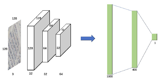
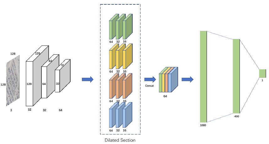
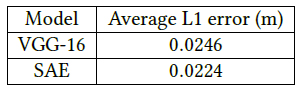
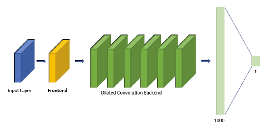
Deep learning regression model for estimating the spatial resolution of an overhead image.
The input is an image and the output is the estimated resolution in meters per pixel.
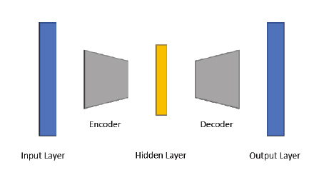
We experimented with different frontends including a standard pretrained CNN and an SAE encoder.

Stacked autoencoder frontend.

The motivation is that the SAE could be trained in an unsupervised fashion to extract features that are more appropriate for our drone imagery than features from a CNN that has been pre-trained on a non-overhead image dataset (such as ImageNet). Indeed, our experimental results show that the regression model incorporating the SAE outperforms our previous model that uses a pretrained CNN:

Results of different frontends. (Lower is better.)

This work was published at the International Workshop on AI for Geographic Knowledge Discovery (GeoAI) at ACM SIGSPATIAL 2019. The paper reviewers and attendees of that workshop found our work on estimating the spatial resolution of overhead imagery novel and interesting.

We also developed a new dataset to train and evaluate our bottom-up approach to estimating the spatial resolution. In the first year, we simulated images with different resolutions by starting with 1 m/pixel imagery and then downsampling it to lower resolutions ranging from 2 to 10 m/pixel. In the second year, we assembled a new dataset 1) with much higher resolution, including 0.15 m/pixel, 0.3 m/pixel, 0.6 m/pixel, and 1.0 m/pixel; and 2) in which these resolutions are native and not resampled. Examples of these images are shown below:

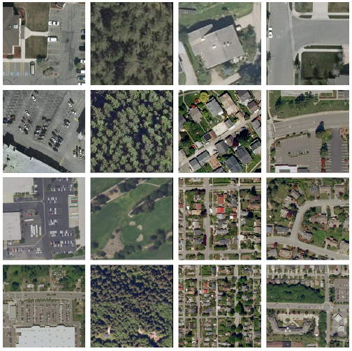
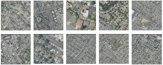
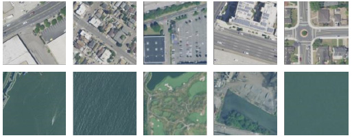
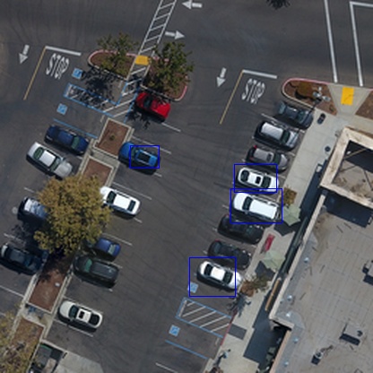
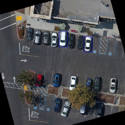
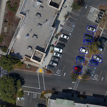
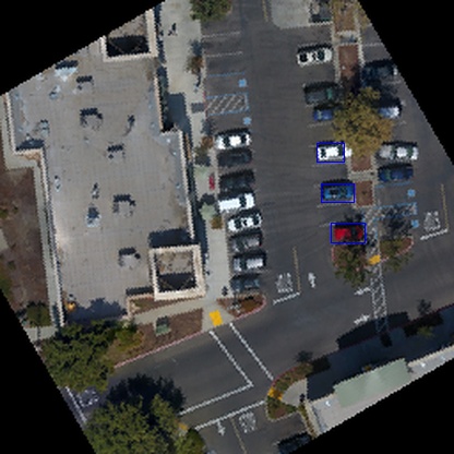
Sample images from our dataset for training and evaluating our bottom-up approach to estimating the spatial resolution.
Columns from left to right depict parking lot, vegetation, housing, and road regions.
Top row: 0.15 meter/pixel images
Second row: 0.30 meter/pixel images
Third row: 0.6 meter/pixel images
Bottom row: 1.0 meter/pixel images.

In the second year, we investigated top-down approaches to estimate the spatial resolution. The goal is to automatically detect objects with (approximately) known size in an image and then use the size of the detected objects to derive the spatial resolution. We focused on detecting cars since 1) they are frequently occurring objects; 2) they tend to have consistent width; and 3) the availability of pre-trained car detectors.

This work has turned into an interesting investigation on using pre-trained object detectors not so much for the sake of detecting object instances but to learn about the imagery itself. In particular, several interesting challenges arose. First, most object detectors, including the one we are using, demarcate detections using a rectangular bounding box oriented with the sides of the image even when the object might not be. (For example, when a car is oriented diagonally, the bounding box is not.) While this makes the design and training of the detector easier since only 4 values need to be estimated for each detection (opposite corners of the bounding box) instead of 5 which would include the angle of the box, it creates a challenge for us since we are using the shortest size of the bounding box to estimate the width of a car. Our solution is to perform car detection on rotated versions of an image and use the statistics (the lower bounds) of the smaller side of the bounding boxes to determine the width of a car when the box fits the car well, that is, when the car is oriented horizontally or vertically in the image. The two images below demonstrate how the bounding boxes are oriented with the sides of the image. The images also demonstrate how performing the detection on rotated version of the image results in detections in which the cars are oriented vertically or horizontally and thus bounding boxes that fit well.

Another challenge is that object detectors tend to have limited scale invariance. That is, they will fail to detect objects when the objects are much bigger or smaller than in the training dataset. Compounding this is that they will provide false positives when there is a scale mismatch. We observed that our car detector started detecting non-car objects (in particular, roof vents) in very high-resolution images. We are addressing this problem by applying the detector at downsampled versions of an image. For the range of scales in which the car detector works, there is a linear relationship between the size of the bounding box detections and the resolution of the image. This linear relationship is broken outside this range. We can use this to determine the resolutions of an image that result in true detections and only use those detections.

The final challenge is that the bounding boxes are somewhat larger than the cars and thus using the size of the smallest side overestimates the spatial resolution. Fortunately, the amount the bounding boxes are larger than the cars is consistent. We are thus addressing this by using a plot of resolution versus smaller bounding box side for calibration. This calibration is easily derived by applying the car detector to training images of known resolution. The following figure shows the relationship between the image resolution and the smaller bounding box side. On the x-axis is the image resolution and on the y-axis is the size of the smaller bounding box side in terms of pixels. The linear region indicates the range of resolutions for which the car detector works.

We expect to use our car detector to estimate the spatial resolution of images as follows. First, we apply the detector to rotated and downsampled versions of the image. We plot the size of the smaller side of the bounding boxes versus downsampling amount (scale). We detect the range of scales where this relationship is linear and use the calibration to estimate the spatial resolution. We are starting to perform these experiments.

Our top-down approach can easily be extended to also use other kinds of object detectors when, for example, images are unlikely to contain cars. The approach will be limited, of course, to images in which objects of standard size are present.

Significant Results:

We extended our bottom-up regression-based approach by using a stacked autoencoder (SAE) to extract improved features for input to the regression model. The SAE can be trained in an unsupervised fashion to extract features that are better suited to overhead images. We demonstrated that this results in improved performance than our earlier framework which used a CNN pretrained on ImageNet to extract the features. We also developed a higher-resolution training and evaluation dataset with images with natively different resolutions and not simulated through downsampling.

We developed a top-down approach to estimating the spatial resolution of an image. We apply an existing car detector and use the size of the detected bounding boxes to estimate the resolution. We overcame several technical challenges including: 1) the bounding boxes only being oriented with the image and not the object; 2) the limited scale invariance of the detector; and 3) the slight overestimate of the object region by the bounding box.

In addition to this top-down approach being useful for the goals of the grant, it was an interesting investigation into how existing object detectors can be used to derive unknown information about images. We expect the computer vision community will find this interesting.

Year Three

Major Activities:

During the third and final year of the project, we finalized our work on estimating the spatial resolution (meters/pixel) of drone imagery. In particular, we focused on a top-down approach in which we first automatically detect objects with a known size and then use these objects to estimate the spatial resolution. We focused on detecting cars since 1) they are frequently occurring objects; 2) they tend to have consistent width; and 3) the availability of pre-trained car detectors.

This work has turned into an interesting investigation on using pre-trained object detectors not so much for the sake of detecting object instances but to learn about the imagery itself. In particular, several interesting challenges arose. First, most object detectors, including the one we are using, demarcate detections using a rectangular bounding box oriented with the sides of the image even when the object might not be. (For example, when a car is oriented diagonally, the bounding box is not.) While this makes the design and training of the detector easier since only 4 values need to be estimated for each detection (opposite corners of the bounding box) instead of 5 which would include the angle of the box, it creates a challenge for us since we are using the shortest size of the bounding box to estimate the width of a car. Our solution is to perform car detection on rotated versions of an image and use the statistics (the lower bounds) of the smaller side of the bounding boxes to determine the width of a car when the box fits the car well, that is, when the car is oriented horizontally or vertically in the image.

Another challenge is that object detectors tend to have limited scale invariance. That is, they will fail to detect objects when the objects are much bigger or smaller than in the training dataset. Compounding this is that they will provide false positives when there is a scale mismatch. We observed that our car detector started detecting non-car objects (in particular, roof vents) in very high-resolution images. We are addressing this problem by applying the detector at downsampled versions of an image. For the range of scales in which the car detector works, we expect a linear relationship between the size of the bounding box detections and the resolution of the image. This linear relationship is broken outside this range. We can use this to determine the resolutions of an image that result in true detections and only use those detections.

The final challenge is that the bounding boxes are somewhat larger than the cars and thus using the size of the smallest side overestimates the spatial resolution. Fortunately, the amount the bounding boxes are larger than the cars is consistent. We are thus addressing this by using a plot of resolution versus smaller bounding box side for calibration. This calibration is easily derived by applying the car detector to training images of known resolution.

We showed this framework is effective for estimating the spatial resolution of drone imagery. We created a set of training and evaluation images with spatial resolutions ranging from 2cm to 32cm per pixel as follows. We started with a 15232 by 15299 pixel image with 2cm spatial resolution that is a mosaic of images captured from a DJI Phantom drone flying at 100m over a site with cars. We then resample this image to have spatial resolutions ranging from 4cm to 32cm in increments of 2cm. We then applied an off-the-shelf object detector (YOLO-v3) that had been trained to detect cars to a training dataset. We used these detections to derive a calibration curve between known spatial resolution and the average width of the bounding boxes of the car detections. As predicted, this detector breaks down when the resolution of the imagery is very high (2-6cm). Somewhat unexpected is that the relationship elsewhere is not actually linear but curved. We therefore fit polynomials of degrees two and three to this calibration curve.

We then applied the same object detector to a set of test images. We applied the detector to the original resolution of these images as well as resampled versions to come up with an observed relationship between these scaling and the sizes of the widths of the detected bounding boxes. We then fit this observation to the calibration curve derived above from the training images using least squares to estimate the spatial resolution of the test image. Our results show that we are able to predict the spatial resolution to within 2cm on most of the test images.